 The space containing
the target is divided into small cubic cells, thus the position
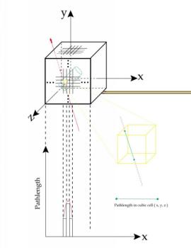
(x,y,z) in this space can be denoted by the position of a cube(nx,ny,nz) enclosing this point.
In above example, nx=int(x/size_of_cell), etc..
The space containing
the target is divided into small cubic cells, thus the position
(x,y,z) in this space can be denoted by the position of a cube(nx,ny,nz) enclosing this point.
In above example, nx=int(x/size_of_cell), etc..From MWPC data, we reconstruct the track of a charged particle, extend this track to go through the fiducial volume enclosing the taget, calculate the 'pathlength' in each cube, and fill the pathlengthes into corresponding cubes in histograms. The pathlength is the length of a segment of the track in a cell. After processing enough numbers of tracks, the accumulated pathlengthes in each cube will reflect the possibility of pions stopping in that cube.
In the meantime, MC method is used to study the output pathlength distributions corresponding to different pion stopping distributions in the target. For each cell size, different Gaussian distributions with different sigmas in target were simulated and the correspondence between stopping distributions and pathlength distributions were plotted and fited with polynomials. The comparison of these polynomials with different cell sizes are showed in the figure in which x is sigma of pathlength distribution, y is sigma of distribution of particles in target.
To determine the center, for a given cell size, we also get the correspondence between the readout center postion and the center of the simulated distribution . The figure is for cell size equal to 1.5 mm.
Compared with the pathlength distribution obtained from experimental data, we can get the corresponding pion stopping distribution.
To do this, with different cell size, we analyzed same set of data, namely from run36030 to run36049, and plotted the obtained pion distribution in the target vs. cell size.
Since the real pion distribution in target is not symmetric, we fitted the data with gaussian_left + gaussian_right
  if(x < center)
    distribution = A*gaussian(center,sig_left)
  else
    distribution = A*gaussian(center,sig_right)
To further test the consistency, with cell size set to 1.5mm, we get sigma_left and sigma_right and center, then we put these parameters back to MC to generate the corresponding pathlength distribution. we then compare the distribution generated in MC with the distribution obtained from the data. The consistency of these two resulted pathlength distributions are well demonstrated. In the Plot of the results, top panel is the distribution in X, bottom is that in Y. the solid line is from MC, the dashed line is from data.
As for the dependence on the fiducial volume, since we only use the pathlenth distribution within a certain range in the current approch to get thereal stopping distribution in the target, the method we are using now is intrinsically independent of fiducial volume.